Introduction
HBComposer is an unofficial tool for pre-processing Hasselblad RAW files. It is able to perform the following 3FR to 3FR operations in the RAW domain:
Frame-Average
Frame-Median
Advanced Flat-Field correction
Since the produced files are still raw files, they can be further processed in any RAW developer, especially in Hasselblad Phocus without losing the advantage of the Hasselblad Natural Color Solution (HNCS). The advanced flat-field correction is able to fix the infamous Hasselblad PDAF banding issue and any sensor tiling artifacts generated by digital backs when used in conjunction with technical cameras and shifted wide-angle lenses.
*** DISCLAIMER *** I am in no way connected to Hasselblad, nor does Hasselblad endorses this project. This tool is the result of my personal initiative and the files produced are not guaranteed to be 100% OEM compliant. Moreover, Hasselblad may change their RAW file specs in any moment causing the tool to stop working.
Product installation and execution
Getting HBComposer
HBComposer is offered for free. You can download it from my web site under the following link:
https://photography.marcoristuccia.com/hbcomposer-an-hasselblad-raw-file-composer/
Support my work
Please consider donating to allow me spend more time in improving it and fix any bugs. Thank you!
Installing HBComposer
The HBComposer installation file is a typical Apple DMG archive. Once downloaded, just double click on it, a window will show up (Figure 2).
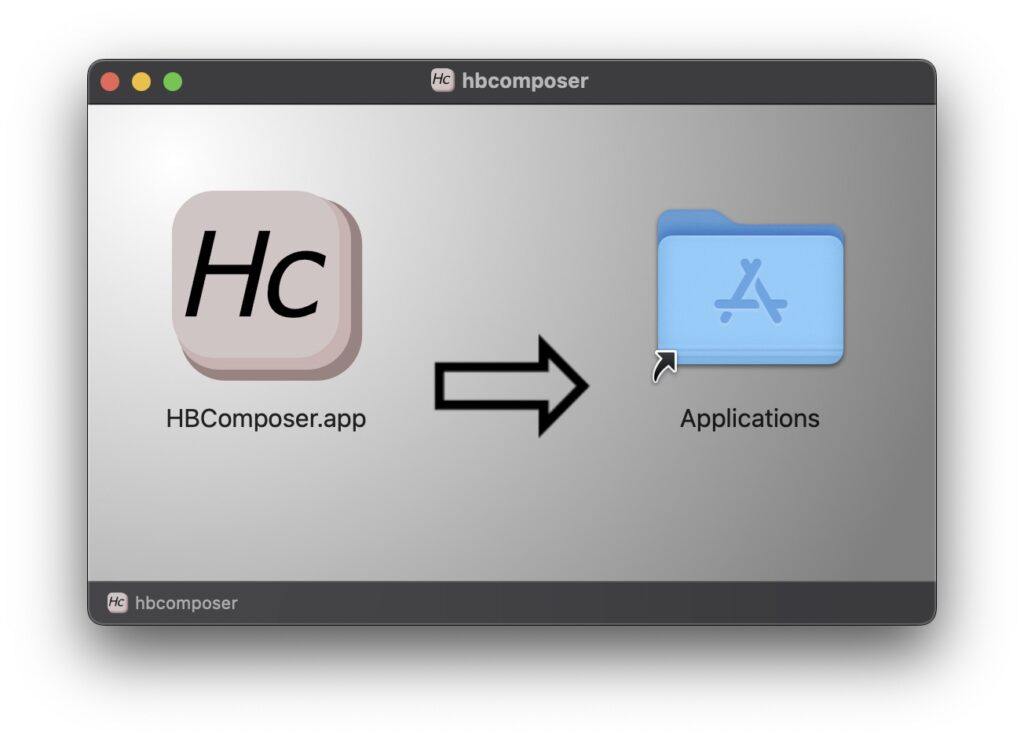
Just drag the HBComposer.app icon onto the Applications one. The application will be installed, if a previous version is already present, macOS will ask whether to overwrite the old version.
Installing Java runtime
To run HBComposer, a Java runtime needs to be installed on your system. The minimum supported version is Java SE 11, although it is highly recommended to install Java SE 21 LTE (Long Time Support) or Java SE 24 (the latest version to date).
You can download Java from the following link:
https://www.oracle.com/java/technologies/downloads/?er=221886#jdk21-mac
Running HBComposer
Once installed, you will find HBComposer among the macOS applications. Just click on it. Please be patient, the application startup may take a few seconds since macOS needs to verify the application and instantiate the Java runtime environment.
Since I’m officially part of the Apple Developer Program, I have digitally signed and notarized HBComposer as per Apple recommendations. Security wise, macOS should not complain about opening it, apart from warning you that the application has been downloaded from Internet and asking for your authorization to proceed.
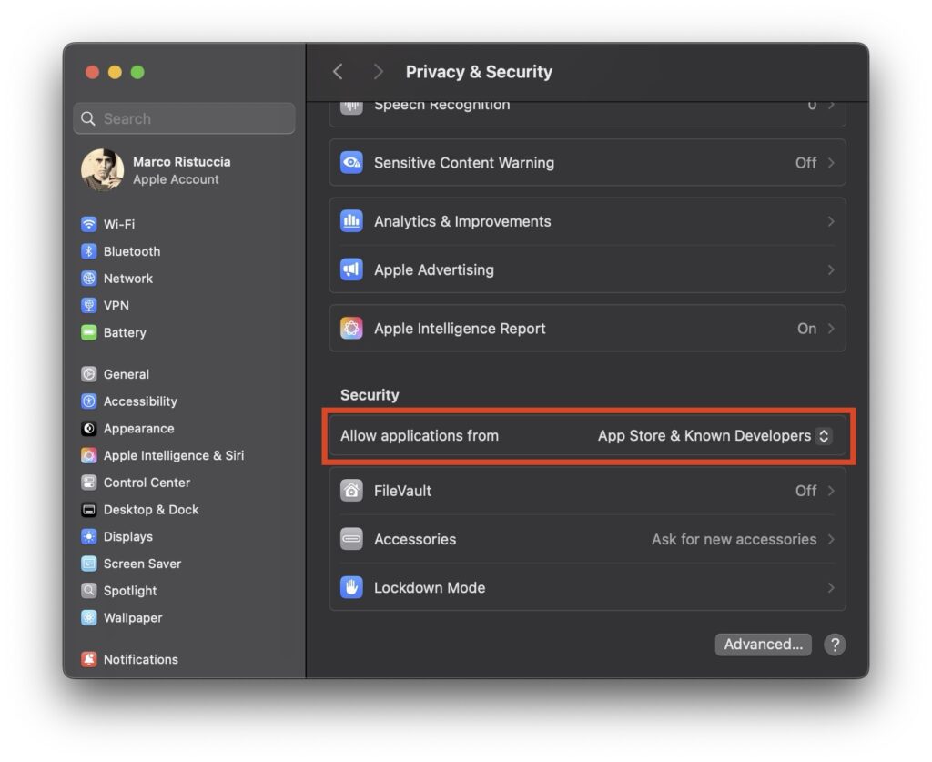
Since the application will not be downloaded from the official Apple Store however, you may need to slightly relax the security settings by allowing applications from “Apple Store & Known Developers“.
Such an option can be found under Settings -> Privacy & Security as shown in Figure 3.
User interface overview
In Figure 4, a screenshot of the main application window is shown.
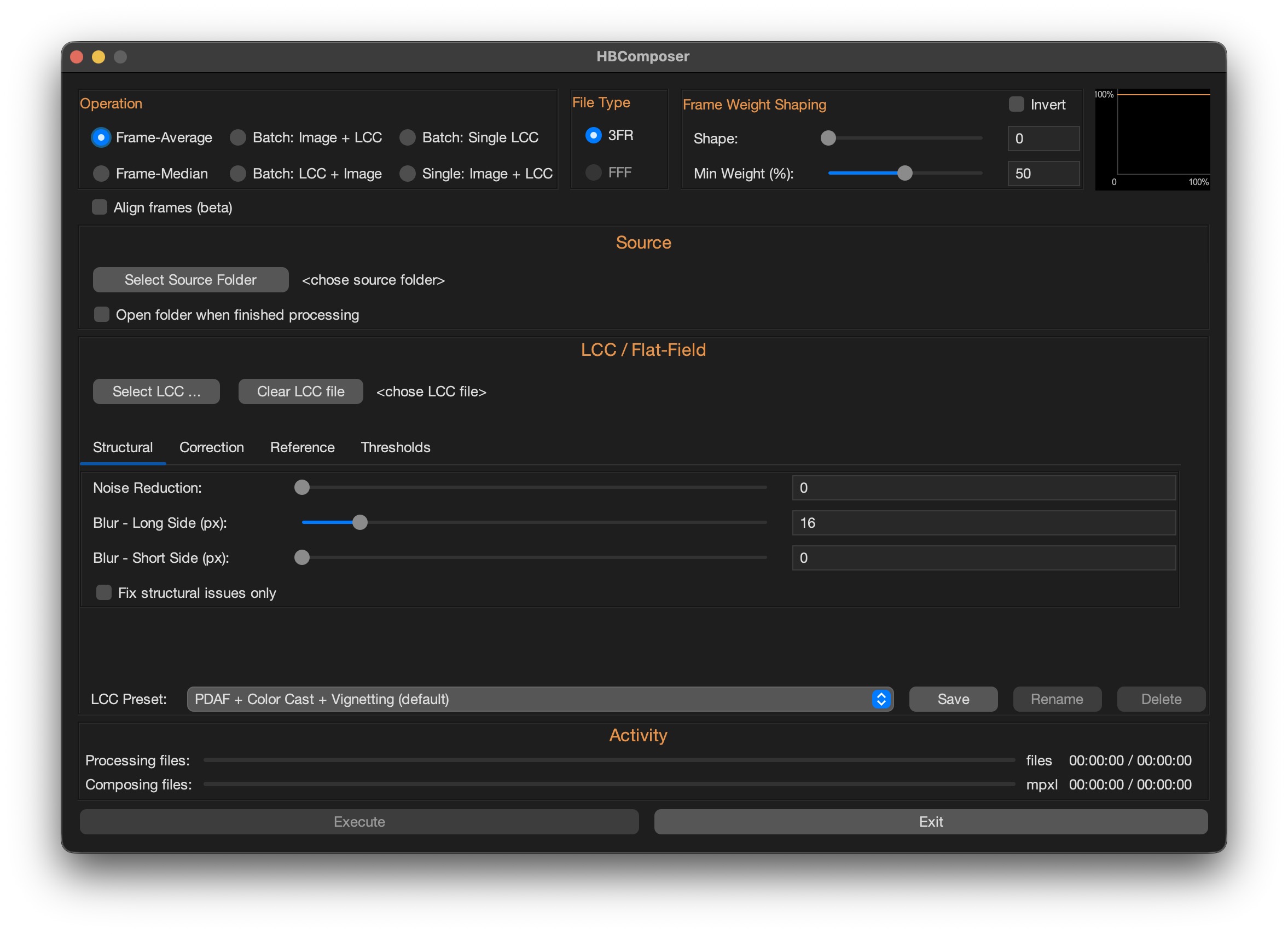
In the following sections, the general configurations are described first. Then, each operation will be fully explained in dedicated sections.
Operation
This area shows available operations to choose from.
See the dedicated Operations below in this document for more details on each operation.
File Type
The tool has been initially designed to operate on both 3FR and FFF Hasselblad RAW files.
Due to technical reasons though, only 3FRs are supported at the moment. For such reason, the FFF option is grayed out and not selectable.
Frame Weight Shaping
This area allows to shape how frames are weighted during a frame-average or a frame-median operation.
See the dedicated Frame Weight Shaping below in this document for more details.
Source (New)
Depending on the chosen type of operation, a button is presented here to select the working file(s).
Files (New)
Used for batch operations. All images to be processed must be selected. You have the option to automatically open the containing folder after the processing is finished.
NOTE: starting from version 1.6.0, the source of batch operations has been switched from entire folder to files selection. From now on, all files to be processed need to be selected instead of the containing folder. This should give more flexibility. It’s important to note that the order in which images are selected matters for the “Batch: Image + LCC” and “Batch: LCC + Image” operations. If a range is selected, images are processed from the first to the last as they are shown in the select window. If you select images one by one, the processing order will follow your selection order.
File
A single image to be processed. You have the option to automatically open the file folder after the processing is finished.
LCC / Flat-Field
In this area a LCC file to be applied to the processed image can be chosen. A set of parameters controls how the LCC correction is performed. See the dedicated section below for more details.
Activity
In the bottom area of the application window there are progress bars that are updated while processing. The composition operations will process files first, then compose them, so both progress bars are updated. The batch LCC operations only update the first progress bar.
Performance parameters
Performance parameters can be accessed by selecting the menu bar HBComposer -> Settings….
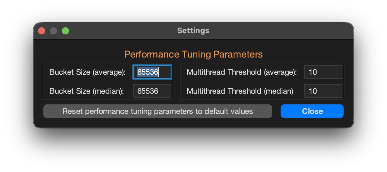
These parameters only apply to the frame-average and frame-median operations.
There is a couple of them for each of the two operations:
Bucket Size
Represents the sliding memory window which buffers the part of the image that is kept in memory while processing the frame compositions. It is represented in bytes. The default value is a good compromise for the majority of systems. If your system happens to have a large amount of RAM (> 36GB) you can try increasing this value (keep it a multiple of 4096). This may speed up the composition operation. Be aware however that you may experience memory over-allocations, in such case the application may slow down or even crash with an unexpected exception. If this happens, just restart HBComposer and reset to the default performance values. If you decide to venture into changing this parameter, you’ll need to find the sweet spot.
Multithread Threshold
Represents the maximum number of parallel processing threads. The default value is a good compromise for the majority of systems. If your system has a large amount of CPU cores (> 14) you can try increasing it. This may speed up the composing operation. If you decide to venture into changing this parameter, you’ll need to find the sweet spot.
NOTE: all performance parameters are remembered after closing and reopening the application. They can be reset to their default values by clicking the dedicated button.
Sidecar files
RAW files are never altered by RAW processors. Instead, changes are either stored in a database (e.g. in Lightroom) or in a sidecar file (e.g. Phocus and Lightroom). Sidecar files created by RAW processors are associated to any edited RAW image and contain all its editing history.
Starting from version 1.4.9 of HBComposer, any sidecar file associated with the source image(s) is replicated and associated to the processed one. This ensures that any edits made to the source image are preserved.
The currently supported sidecar types are:
XMP (.xmp): created by Adobe Lightroom when the flag for creating them is enabled in LR settings.
PHOS (.phos): Created by Hasselblad Phocus starting from version 4 when editing 3FR RAW images instead of FFFs.
NOTE: for frame-average and frame-median operations, the sidecar files of the first image of the source sequence are the ones that will be replicated and associated to the final processed image.
Operations
Frame-Average
This operation will perform a composition of all images found in Source Folder, producing a single RAW image which represents a pixel-by-pixel average of all processed images. The output file will take the name FA.3FR and is automatically ignored by all operations, so you can keep it there and re-run frame-average or frame-median without it to be part of the composition. It will be simply rewritten.
In a typical situation, you place your camera on a tripod and use the featured internal intervalometer to shoot a series images of the same scene at a specified time cadence.
Figure 6 presents an example of the results that can be achieved with frame-average.
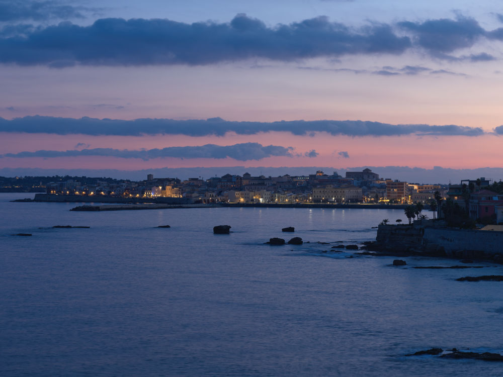
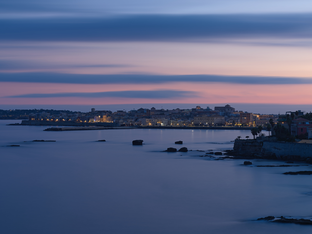
It shows the result of a frame-averaged composition of 160 frames, each one shot at ISO 64, f8 and 0.8s exposure time without any ND filter. It produced a RAW image which is roughly equivalent to a 2-minutes long exposure taken with an 8-stops ND filter on.
Frame-Average may be useful for the following purposes:
It reduces the overall image noise, especially in the shadows.
Noise is reduced by the square root of the number of frames averaged. So, if you average 4 images, noise will be reduced to 1/2 of the noise you’d have in a single frame.
On moving subjects, it produces an effect similar to a long-exposure.
An advantage to a real long-exposure is that you can operate in daylight without the need of an ND filter.
A disadvantage is that Hasselblad cameras do not currently allow shooting images at a speed greater than one frame every two seconds. Thus, fast moving objects may not be represented as a continuous trail in the final composed image. To try to partially compensate for this issue, an frame weight shaping function has been added to the tool (see below for more info on this).
Another tip to reduce gaps between frames to the minimum is using a remote cable trigger with a lock button, this will avoid the 2 seconds gap the camera intervallometer would introduce.
Frame-Median
This operation will perform a composition of all images found in the Source Folder, producing single RAW image which represents a pixel-by-pixel median of all processed images. The output file will take the name FM.3FR and is automatically ignored by all operations, so you can keep it there and re-run frame-median or frame-average without it to be part of the composition. It will be simply rewritten.
In a typical situation, you place your camera on a tripod and use the featured internal intervalometer to shoot a series images of the same scene at a specified time cadence.
Figure 7 presents an example of the results that can be achieved with frame-median.
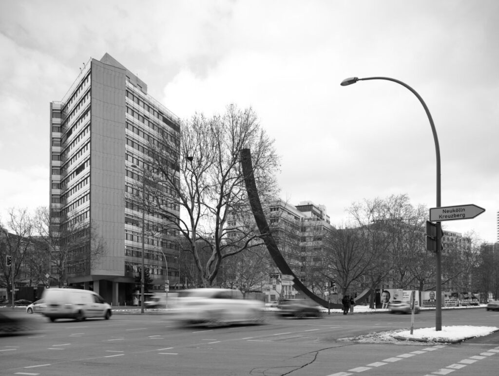
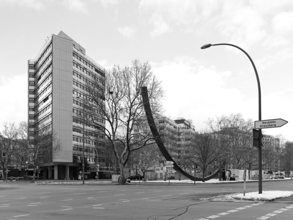
It shows the result of a frame-median composition of 34 frames, each one shot at ISO 64, f8 and 1/10s exposure time without any ND filter.
As shown in the sample image, on scenes containing moving objects like cars, persons, etc… frame-median may be useful to cancel them out from the final image. A crowded place where many people pass by can be turned into an empty space. This can be useful for example in architecture photography.
Like with frame-average, frame weight shaping could help in smoothing out some gaps, like on moving clouds for example, although it will increase the calculation time (see an example of weight shaping results below in the dedicated section).
Another tip to reduce gaps between frames to the minimum is using a remote cable trigger with a lock button, this will avoid the 2 seconds gap the camera intervallometer would introduce.
Frame Alignment (New)
Option Align frames only applies to frame-average and frame-median operations. When activated, it tries to align frames before they get composed. This may be useful if vibrations due to the wind or a flimsy tripod+head combo may have caused a slight misalignment of the captured frames.
Since the alignment occurs in the RAW domain, only displacements with an even number of pixels can be recovered. Currently, the algorithm can correct displacements of up to 32 pixels in the RAW domain.
Due to the RAW nature of the treated image, only horizontal and vertical shifts are treated. Fixing rotational displacements would break the RGGB alignment and would require pixel interpolation/reconstruction in the RAW domain, which could be more detrimental than beneficial. Better to use a sturdy tripod!
Please note that frame alignment will slow down the composition process. All misplacements are calculated at the beginning of the composition process. So, you will notice a delay when the pre-processing progress bar is near the end.
NOTE: this feature is still in beta version.
Frame Weight Shaping
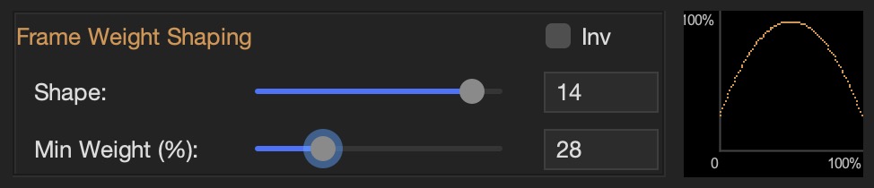
You’ll find this option in the top-right area of the application window. This feature shapes the weight of the frames in different ways while performing frame-average and frame-median. This feature may help in smoothing out some gaps that may arise in presence of moving objects in the scene when the time interval between captured frames is long.
Shape
selects the curvature of the shaping function.
Weight Perc (%)
selects the minimum weight value in percentage (maximum is always 100%).
Inv.
inverts the shaping function.
The live graph on the right will live preview the shaping function while its parameters are changed.
In Figure 9 you’ll find a result comparison based on a frame-median composition of 100 images shot at a frequency of 1 every 10 seconds. Without weight shaping (left), gaps in the clouds are visible in the upper and central right part of the image. Weight shaping succeeded in smoothing things out (right).

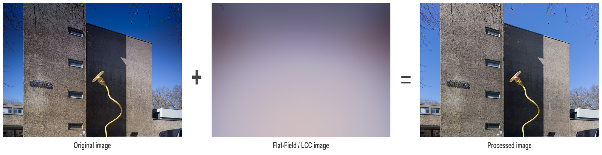
Flat-Field Correction
HBComposer features a flat-field correction operation and offers an advanced set of fine-tune parameters.
This technique consists in taking an additional frame, called flat-field or LCC, while holding a thick piece of white semi-transparent plexiglas in front of the lens. This special image should be acquired under the very same conditions as the photo it will correct. Aperture, focus, shift/tilt levels, and light conditions need to match. Shutter duration can be adjusted to get a correct exposure. A good LCC exposure is key to the effectiveness of this technique.
From now on, the words flat-field and LCC will be used alternatively to indicate this special frame.
Figure 10 shows a typical histogram of a well exposed flat-field image. To minimize noise transferred to the processed image, it must be exposed to the right without cropping the highlights (ETTR).
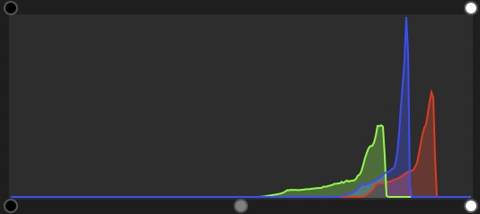
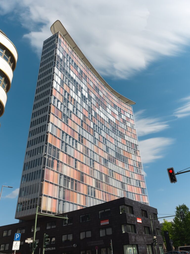
Figure 11 shows a typical example of a flat-field image taken with a technical camera and a shifted (raised) lens.

Figure 12 explains how the LCC correction process works. The flat-field capture is applied to the original image to normalize it.
Goals of flat-field correction
Flat-field correction allows the reduction and often the full elimination of the following image issues:
Color cast when taking images with shifted lenses. The issue is particularly evident on non-BSI sensors when used in conjunction with symmetrical wide angle and ultra wide-angle lenses, such as the Schneider-Kreuznach technical ones, and some Rodenstocks as well.
Vignetting when taking images with shifted lenses. The issue is particularly evident if using symmetrical wide angle and ultra wide-angle lenses, such as the Schneider-Kreuznach technical ones, and some Rodenstocks as well.
PDAF sensor banding, an issue that has been discovered by GetDPI forum member @diggles while using use the most recent Hasselblad CFV-100c digital back together with a Schneider-Kreuznach Apo-Digitar 5.6/35 XL lens. It shows up when shifting this lens, especially on uniform areas like the sky. In Figure 13 an example of PDAF banding fix performed by HBComposer’s flat-field correction is presented.


Figure 13. (a) Original image – horizontal PDAF banding and vignetting present (b) Processed image – horizontal PDAF banding and vignetting corrected You can follow the forum discussion under the following link (click on it):
https://www.getdpi.com/forum/index.php?threads/hasselblad-100c-and-35xl.75781/
Figure 13 shows an example of PDAF banding fix performed by HBComposer’s flat-field correction.Sensor tiling, an issue which makes evident in the final image the different tiles a digital sensor is typically composed of. The issue is particularly evident on non-BSI sensors when used in conjunction with symmetrical wide angle and ultra wide-angle lenses, such as the Schneider-Kreuznach technical ones, and some Rodenstocks as well. In Figure 14 an example of sensor tiling fix performed by HBComposer’s flat-field correction is presented.
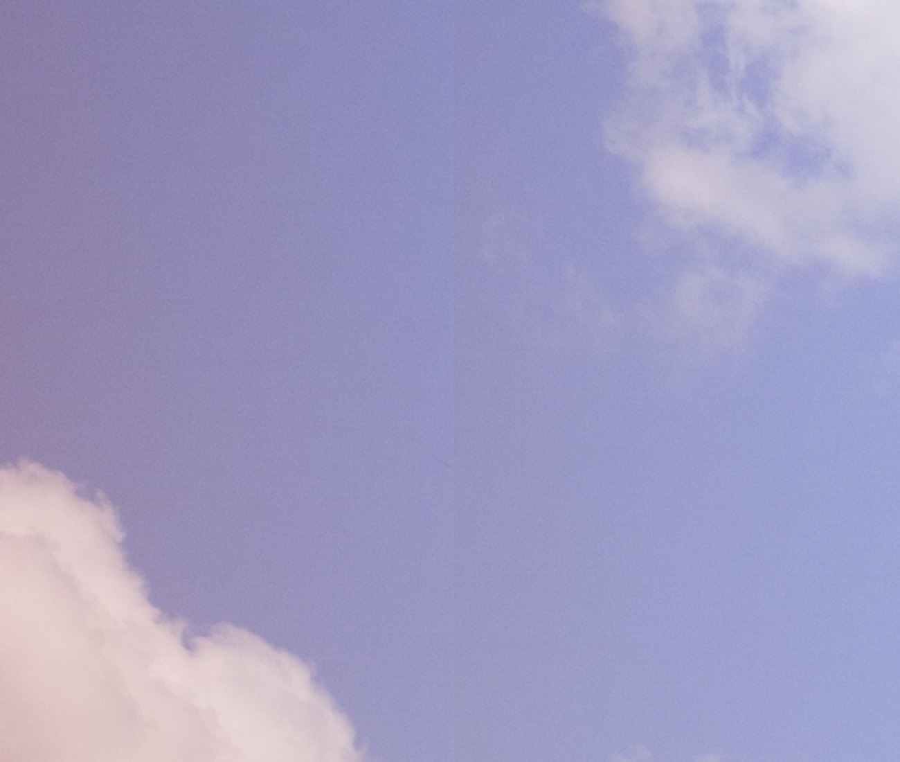

Figure 14. (a) Original image – sensor tiling, color cast and vignetting present (b) Processed image – sensor tiling, color cast and vignetting corrected Dust spots present on the sensor glass which are visible in the final image as darker circular or elongated shapes. In Figure 15 an example of dust spot fix performed by HBComposer’s flat-field correction is presented.
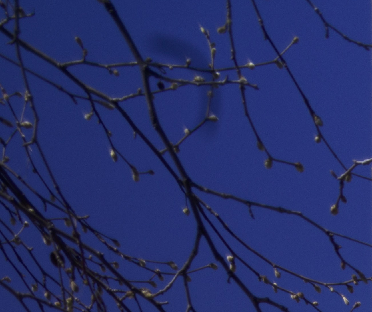
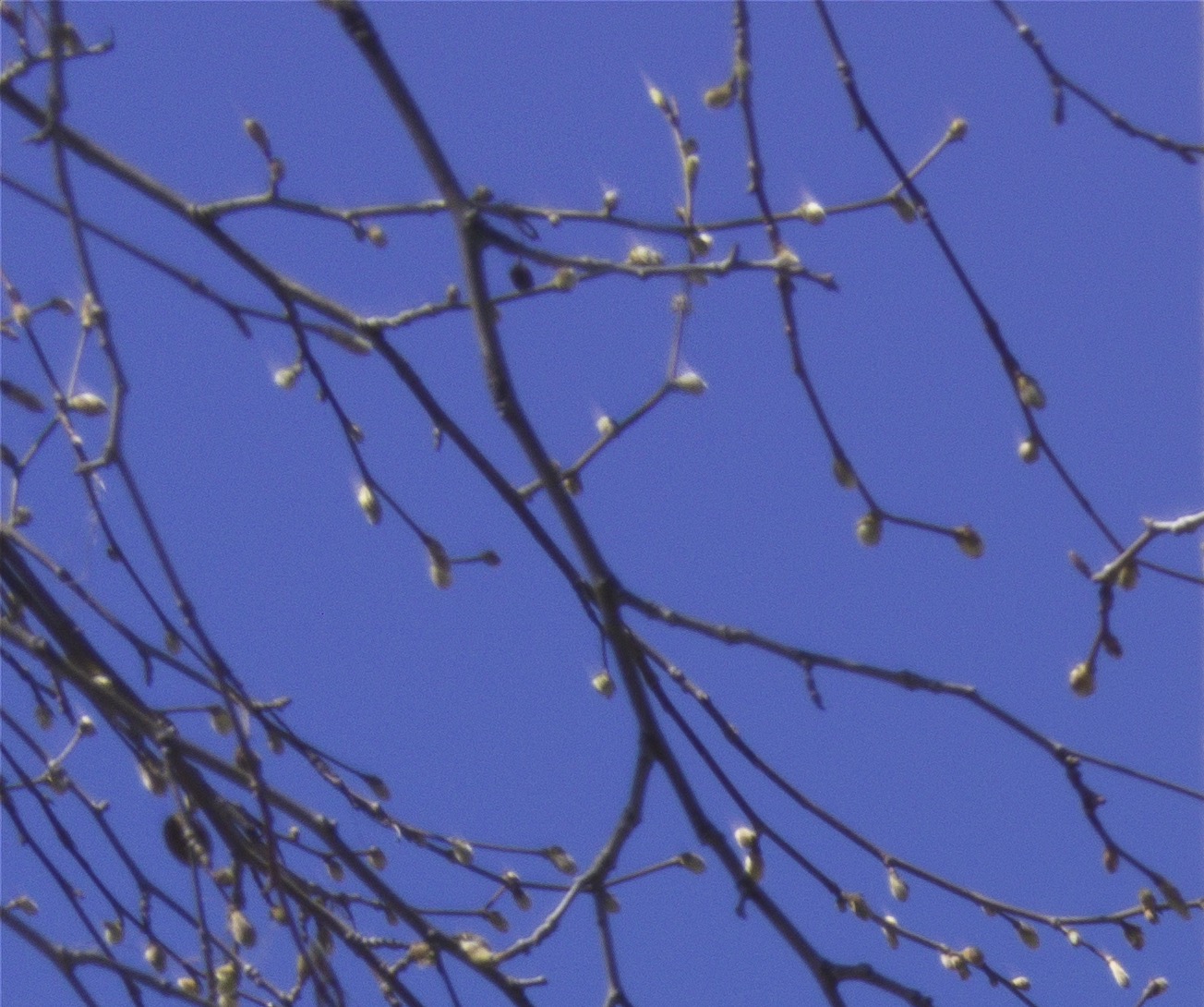
Figure 15. (a) Original image – dust spot and vignetting present (b) Processed image – dust spot and vignetted corrected
IMPORTANT NOTE: unfortunately, in case of extreme vignetting or CA the flat-filed algorithm will not be able to correct everything. High noise and residual color casts need to be corrected later on in the image processing chain, in the RAW developer or in post-production.
Operations and flat-field correction
You can apply a flat-field correction to the following operations:
Frame-Average and Frame-Median
In such cases, the flat-field correction is applied to the final composed image before saving it to disk.
Select the LCC file and adjust all the parameters before executing the composition.
*** NOTE: the LCC file must not be placed in the Source Folder together with the images to be composed, If it is put there, it will be included in the composition as an additional frame. You can place it in a sub-folder instead so that it won’t be composed but only applied at the end.
Batch: Image + LCC or LCC + Image
In this case, images in Source Folder need to be arranged in couples so that, when alphabetically sorted, each LCC frame will immediately follow (Image + LCC) or precede (LCC + Image) its target image.
The corrected images produced by HBComposer will keep the original name with the additional _HBC suffix.
Batch: Single LCC
A single LCC is applied to all files present in Source Folder. In such case, you need to manually select the LCC image as you would do with frame-average and frame-median.
The corrected images produced by HBComposer will keep the original name with the additional _HBC suffix.
Single: Image + LCC
A chosen LCC is applied to a chosen image. The corrected images produced by HBComposer will keep the original name with the additional _HBC suffix.
Flat-field correction modes
Starting from version 1.3.0b, HBComposer offers two ways of applying the LCC to a RAW image:
Correction of structural anomalies only
It only tries to fix PDAF banding, sensor tiling and dust spots. Usually, such anomalies are not addressed by the flat-field correction implemented in RAW developers like Hasselblad Phocus and Adobe Lightroom. After you’ve performed this step through HBComposer, you’ll need to re-apply the LCC through such applications to correct color casts and vignetting, as you would do in normal circumstances. This allows for maximum flexibility.
With this correction mode a large blur radius close to 64 or even greater is recommended. A bit of noise reduction may also help but usually it is not necessary (see below for more details on noise reduction).
Full LCC correction
It tries to fix all anomalies: PDAF banding, dust spots, sensor tiling, color cast and vignetting. After this step LCC correction is fully done and you won’t need any further assistance from external RAW developers to complete the correction.
With this correction mode, a blur radius close to 0 is recommended to fix PDAF banding and sensor tiling. Since the recover of vignetting increases the noise level, a bit of noise reduction (level 2 or 3) is also suggested to get clean results (see below for more details).
Flat-field correction settings
HBComposer offers a set of fine-tuning parameters for flat-field correction. The most useful combinations are provided as factory presets. You can tailor the parameters to suite your use-cases and save them as additional presets.
Parameters are organized in different panels. Here below a brief description of each setting is given:
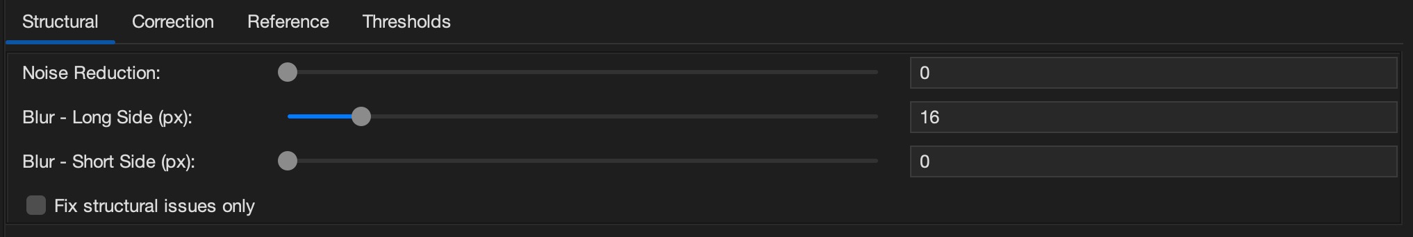
Fix structural issues only
Found under the Structural panel (see Figure 16). As described above, this flag selects the flat-field mode. When enabled, it restricts the correction process to PDAF banding, sensor tiling, and small dust spots only. Color cast and vignetting need to be fixed through an external RAW developer and its LCC correction abilities.
This flag is disabled by default, so HBComposer will normally perform a full LCC correction.
NOTE: when enabled, this option will increase the execution time due to the large blurring radius that needs to be applied.
Noise Reduction
Found under the Structural panel (see Figure 16). Applies a bilateral noise reduction to the final RAW image which is proportional to the level of vignetting recovery performed by the flat-field correction. This clever way of applying noise reduction will be more aggressive in the areas that need it most, while excluding the areas untouched by LCC correction.
A radius of 2 or 3 is usually enough for light to medium degraded LCC images. A value larger than this may be necessary for extremely degraded ones.
This setting is mostly needed when using the full flat-field correction mode (flag “Fix structural issues only” deselected) since in this mode vignetting is recovered by HBComposer. If you only fix structural issues, then noise reduction should be performed by the RAW developer used to complete the flat-field correction.
Blur (long / short side)
Found under the Structural panel (see Figure 16). Sets the pixel radius of LCC blur along each side of the frame. This setting has two different meanings and consequent behaviors depending on the selected LCC correction mode:
“Fix structural issues only” option disabled
Increasing it will reduce the noise in the final image, but it will also reduce the correction effectiveness of structural image issues like dust spots, sensor tiling and PDAF banding.
For PDAF banding correction, keep the “Short Side” blur radius set to 0px and use a “Long Side” blurring radius of 8-16px. This will be still effective in correcting banding while keeping the noise low in the final image. For other structural issues, achieving the perfect compromise between noise and corrections will require some experimentation.
Default values are set for PDAF banding correction: 16px for the long side and 0px for the short side.
“Fix structural issues only” option enabled
Sets the blur pixel radius of the LCC image when applied to itself before being used to fix the RAW image. As opposed to the preceding case, here the blur value must be high (64 pixels or larger) to correct PDAF banding and sensor tiling.
Default values are set to 64px for both the long and the short side.
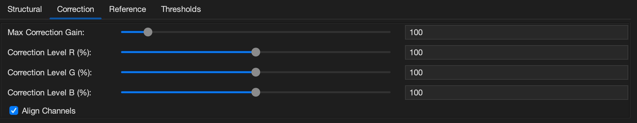
Max Correction Gain
Found under the Structural panel (see Figure 17). The flat-field correction algorithm calculates an amplification factor for each pixel of the target image. This setting defines its maximum (peak). The algorithm will cap the amplification factor to this value. Normally, it can be kept high. You may need to lower it down in case of clipping.
If unsure, leave it at its default value (100), or even 1000.
Correction Levels (R, G, B) (%)
Found under the Structural panel (see Figure 17). Sets the percentage of LCC correction to be applied on each color channel. Normally it should be kept at 100%. You may increase it together with the other channels to over-correct, or decrease to under-correct. If the three sliders are disjoined and set differently from each other, this correction can help in fine-tuning any global color cast, especially if the chosen reference point is not perfectly neutral (see below).
If you still see some banding or sensor tiling, especially when only fixing structural issues, you may want to increase the correction percentage.
The Max Correction Gain caps the maximum amplification factor resulting from this setting.
If unsure, leave the three levels aligned and at their default value (100%).
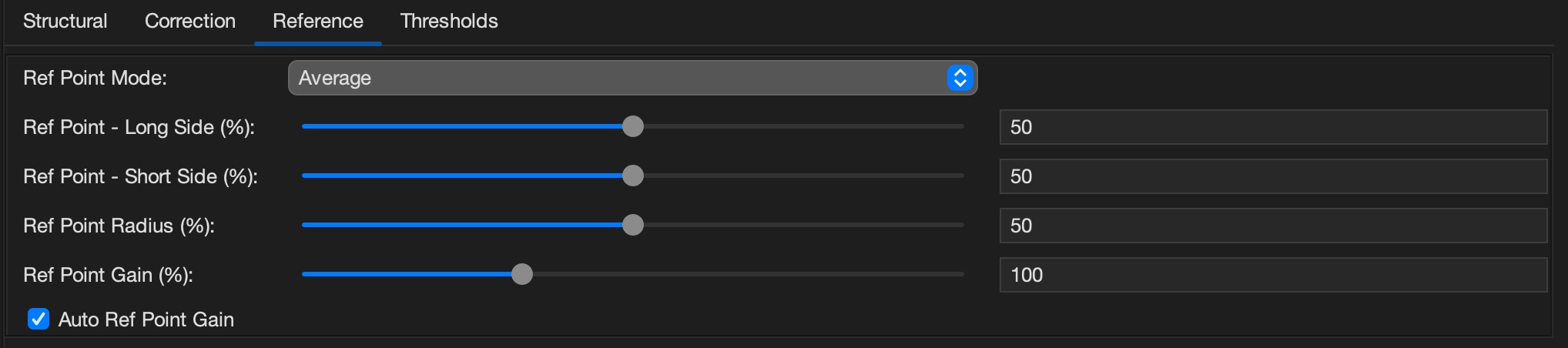
Ref Point Mode
Found under the Reference panel (see Figure 18). The flat-field correction algorithm needs a reference value taken from the LCC image which will be used to normalize the final image in terms of colors and brightness. It sets the values (one for each RGGB channel) where amplification factor is considered to be 1. To over-simplify the matter, you can consider it as the white balance point. This setting allows to choose different ways of calculating it:
Average
The average of the full LCC image is used.
In presence of high vignetting, it may produce a dark image, which you can try to counter balance by using the Ref Point Gain setting (see below),
When a high color cast is present in the LCC frame, the full average may leave some residual global color cast in the final image. In this eventuality, you can disjoin the Correction Levels (R, G, B) % sliders and try to counter-balance the color cast.
If some (under) clipping in the final image happens (usually pink areas), try to increase the Ref Point Gain (see below).
In presence of any of the above problematic cases however it is advisable to switch to Custom Selection mode and manually choose a good neutral LCC point/area.
This is the default selection.
Custom Selection
Offers the option of selecting a specific point of the LCC (Ref Point Radius = 0) or a circular averaged area (Ref Point Radius is > 0). This kind of selection works best in cases where a significant degradation in a zone of the LCC image is present. Just place the reference point/area so that it keeps the degraded zone excluded (see Ref Point (long/short side) (%) and Ref Point Radius (%) below).
Ref Point (long / short side) (%)
Found under the Reference panel (see Figure 18). These sliders are active when LCC Custom Selection mode is selected. They help positioning the reference point along the X-Y plane in percentage values, like shown in Figure 19.
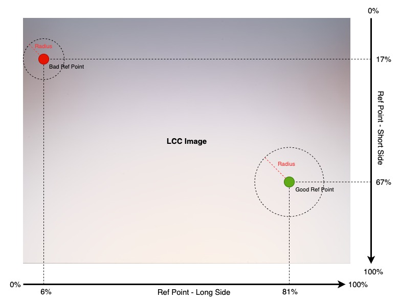
If unsure, leave the Ref Points to the default value (50%, 50%). This places the reference point at the very center of the LCC frame, which works well on average use-cases that usually only have a slight amount of peripheral aberrations.
NOTE: unfortunately, the tool does not feature a live preview of the reference point/area placement nor of the LCC correction results. Multiple attempts may be needed to nail the right spot.
Ref Point Radius (%)
Found under the Reference panel (see Figure 18). When Ref Point Mode is set to Custom Selection, HBComposer offers the possibility of increasing the area around the chosen reference point. The area will cover a circle of a specific radius (percentage) around it. A radius of 0% corresponds to the very single reference point. The maximum radius (100%) corresponds to a circle around the reference point having a radius of half the diagonal of the flat-field image. Values within the area will be averaged.
If unsure, leave the radius at its default value (50%).
Ref Point Gain (%)
Found under the Reference panel (see Figure 18). In some situations, usually in presence of a highly degraded flat-field image, and especially when including severely vignetted areas in the LCC reference area, the produced image may result dark. Increasing Ref Point Gain (%) may help bring the produced image to the right exposure level. This is particularly important in presence of clipped highlights in the source image. Such areas must remain clipped also in the processed image, otherwise they will turn pink due to the absence of color information. If you encounter a similar situation, either manually increase this parameter until you don’t get pink cast on highlights in the processed image (even when lowering down exposure in RAW developers) or enable the Auto Ref Point Gain (see below) to let HBComposer automatically set the gain level for you. If unsure, leave it at its default value (100%) and enable Auto Ref Point Gain.
Auto Ref Point Gain
Found under the Reference panel (see Figure 18). When on, this flag automatically calculates the Ref Point Gain (%) value described above so that the top image highlight value matches the one of the original image. This is very important in presence of source images with clipped highlights, as such highlights must stay clipped in the processed image. If they don’t, they will get a pink cast due to the loss of color information.
After processing the image, the gain calculated automatically will be reported to the Ref Point Gain (%) slider, so that it can be fine tuned manually if necessary. As long as this flag remains on, the value reported on the slider is ignored. Any manual intervention to the slider will automatically disable the flag.
This flag is active by default, as it is also useful for images without clipped highlights because it keeps them at almost the same exposure of the original image,
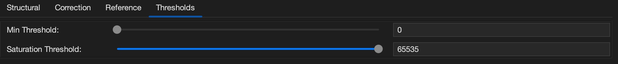
Min Threshold
Found under the Thresholds panel (see Figure 20). Sets the minimum threshold value to consider a pixel of the LCC image valid for correction (0-65535). A value below this threshold leaves the matching pixel of the final image uncorrected.
Normally, Hasselblad RAW files have a black level set to 4096, so anything below that would perform a full correction. You may need to increase it above 4096 if the sensor has some defective pixels that would create problems in the final image. This is really rare though.
If unsure, leave it at its default value (0).
Saturation Threshold
Found under the Thresholds panel (see Figure 20). Sets the maximum threshold value to consider a pixel of the LCC image valid for correction (0-65535). A value above this threshold leaves the matching pixel of the final image uncorrected.
Normally Hasselblad RAW files have a maximum pixel level set to 65535. You may need to decrease this setting below that if the sensor has some defective pixels that would create problems in the final image. This is really rare though.
If unsure, leave it at its default value (65535).
Flat-Field (LCC) Presets (New)
Starting from version 1.5.0, HBComposer supports LCC presets.

In order not to loose your latest settings, when this new version is opened for the first time, it will save them as a custom user profile with name Custom LCC Preset 1 and selects it as current profile.
From that moment on, you can create (save), rename, and delete profiles to your liking.
HBComposer comes with a predefined set of factory profiles which cover the most important use-cases. Here below the list of the factory presets with a brief explanation:
PDAF + Color Cast + Dust + Tiling (best correction, noisy)
Noise Reduction: 0 | Blur Long Side: 0 | Blur Short Side: 0
Corrections: color cast, vignetting, PDAF banding, sensor tiling, dust spots
This is the most effective preset for correcting all issues. Since the LCC image is not blurred at all, this setting will introduce a bit of noise to the processed image(s).
PDAF + Color Cast + Dust + Tiling (with noise reduction, softer)
Noise Reduction: 2 | Blur Long Side: 0 | Blur Short Side: 0
Corrections: color cast, vignetting, PDAF banding, sensor tiling, dust spots
Like the preceding one, but with a bit of noise reduction applied to the processed image, This reduces the noise introduced by the application of the unblurred LCC. The noise reduction is applied proportionally to the vignetting magnitude, it will be stronger on the areas that receive the biggest exposure compensation. There is no such thing as a free lunch though: the noise reduction will introduce a slight loss of micro-details.
PDAF + Color Cast + Vignetting (default)
Noise Reduction: 0 | Blur Long Side: 16 | Blur Short Side: 0
Corrections: color cast, vignetting, PDAF banding
It applies an LCC blurring along the long side, the direction of the PDAF banding. This is still very effective for correcting PDAF banding while minimizing the noise introduced to the processed image. Results on dust spots and sensor tiling may vary. This preset represents the sweet spot for correcting PDAF banding together with color cast and vignetting.
Color Cast + Vignetting
Noise Reduction: 0 | Blur Long Side: 64 | Blur Short Side: 64
Corrections: color cast, vignetting
Applies a blurred LCC image just like any other RAW developer would do. It corrects color cast and vignetting, does not introduce noise, but it is not effective against PDAF banding, sensor tiling and dust spots.
Only Structural Issues
Noise Reduction: 0 | Blur Long Side: 64 | Blur Short Side: 64
Corrections: PDAF banding, sensor tiling, dust spots
This preset activates a special algorithm which only corrects structural issues but does not correct color cast and vignetting. The LCC must be re-applied in your preferred RAW developer to correct them as one would normally do without HBComposer. The idea behind this preset is that commercial RAW developers may do a better job and may have more options than HBCoomposer in doing the usual LCC correction. So, HBComposer can only do what they won’t: correct the structural issues. LCC blur is set to 64px in this case, but it has another meaning/behavior in this special case (Flat-field correction modes, Blur (long / short side)).
NOTE: Factory presets cannot be renamed nor removed.
HBComposer Plugin for Adobe Lightroom (New)
Starting from version 1.5.2, HBComposer comes with a plugin companion for Adobe Lightroom Classic which supports the following actions:
Frame-Average
Frame-Median
Flat field application on Image -> LCC sequence
Flat field application on LCC -> Image sequence
To perform such actions, the plugin communicates with the main HBComposer application, but there is no need to keep HBComposer running. The plugin will invoke it behind the scenes when necessary.
Plugin installation
The plugin is installed via HBComposer:
Launch HBComposer.
Open the Help menu and select Install Lightroom Plugin… (see Figure 22).
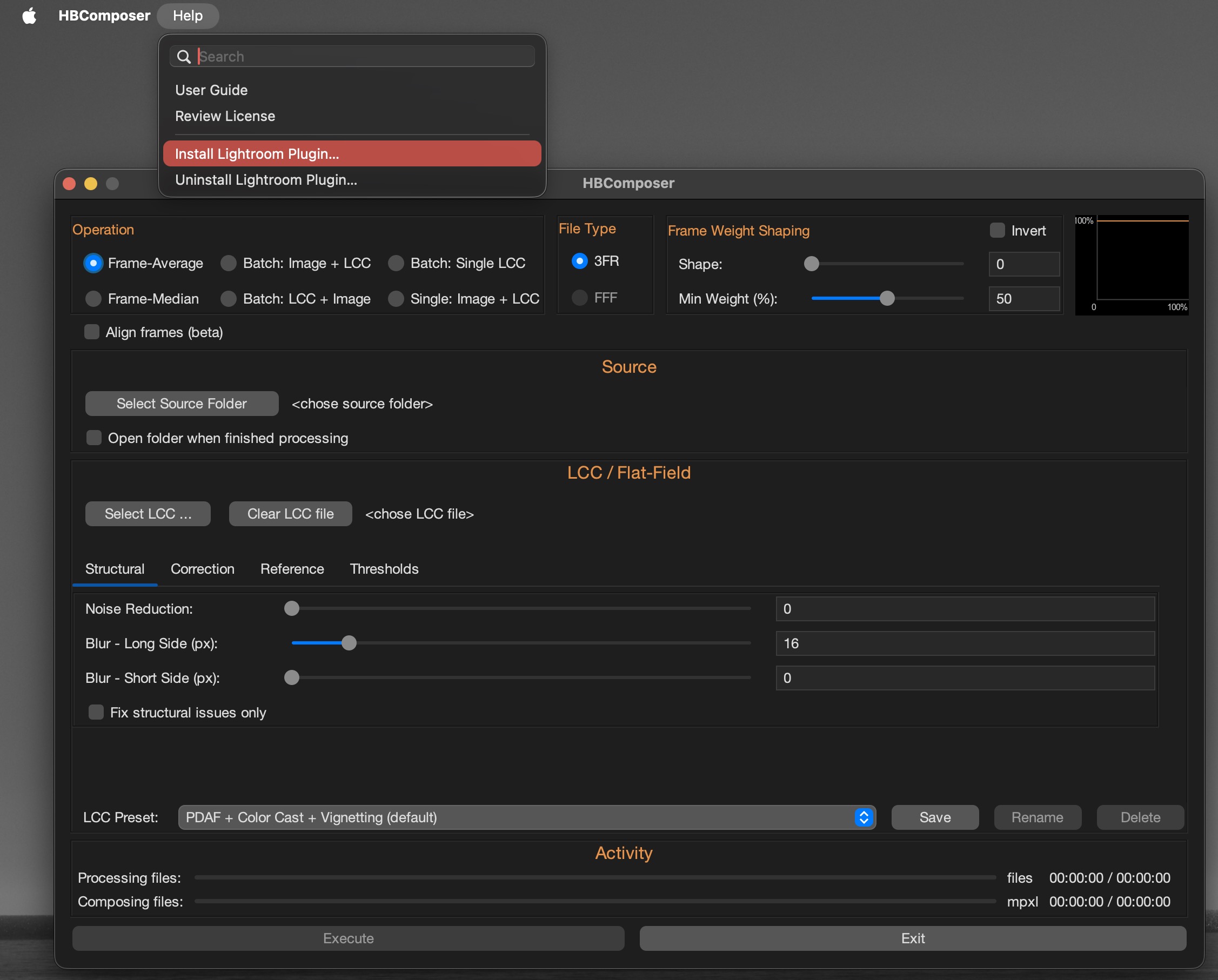
Figure 22. HBComposer – Install Lightroom Plugin The plugin will be automatically installed. If an older version is already present, it will be updated. A dialog box will confirm the installation/update and will indicate the folder where it has been installed (see Figure 23).
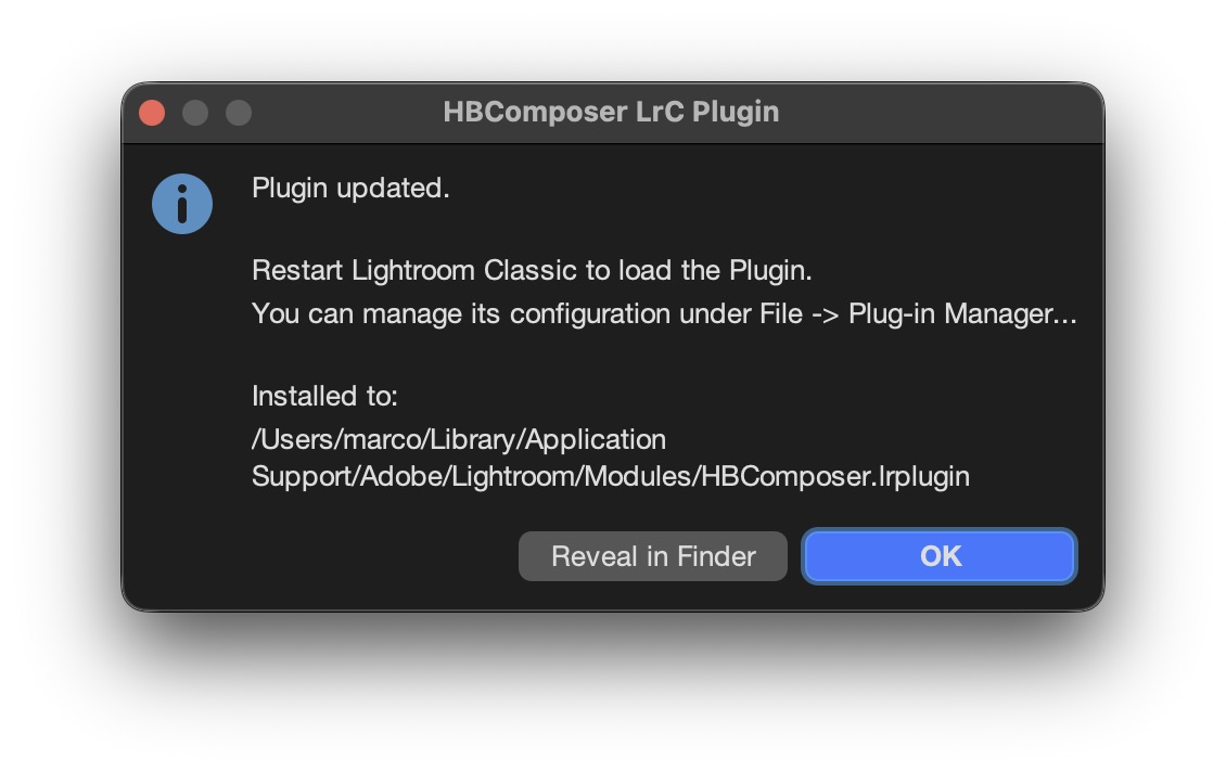
Figure 23. HBComposer – Plugin Installation Result TO complete the installation, A Lightroom restart is needed if it was already running while installing the plugin.
Plugin configuration
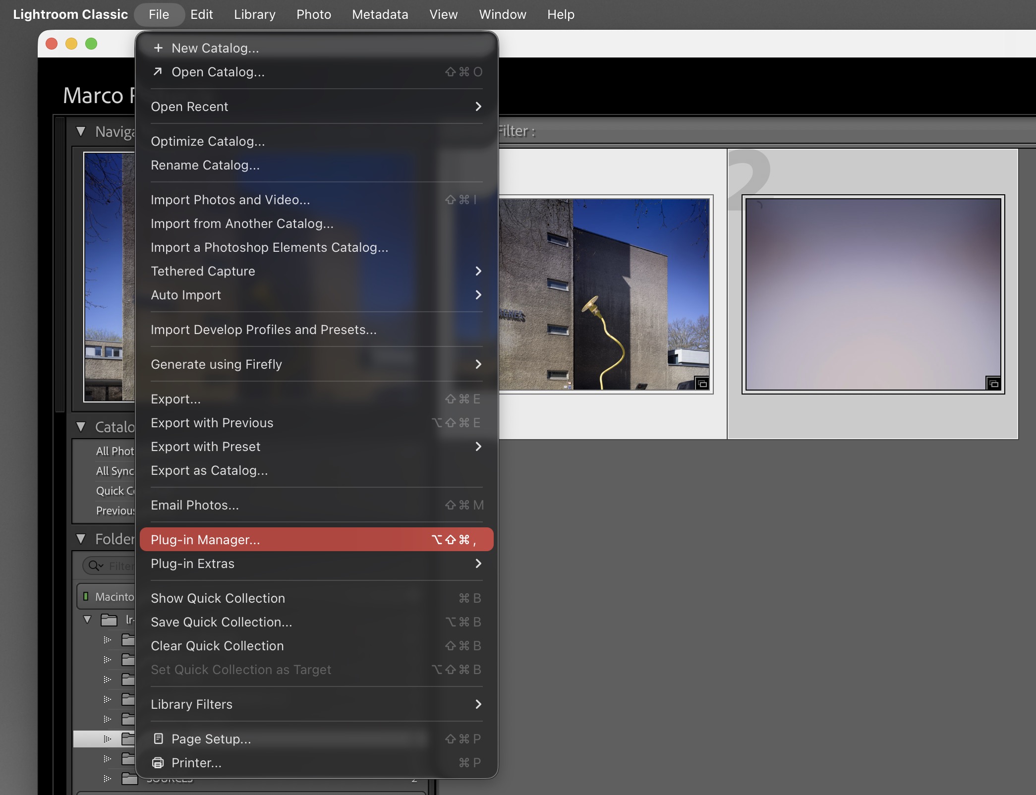
You can enable, disable and configure the plugin in Lightroom by going to Files -> Plug-in Manager… as indicated in Figure 24 and Figure 25.
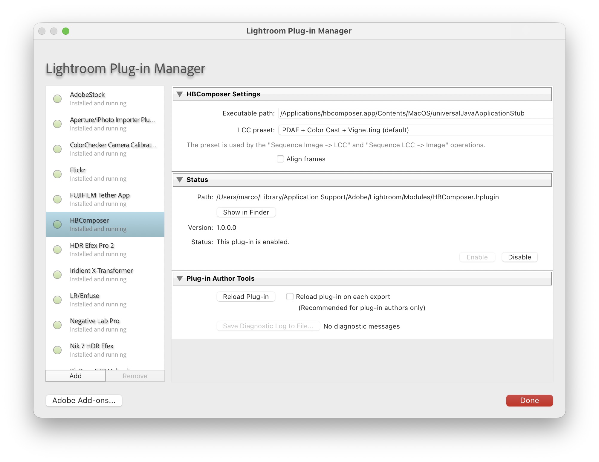
Configuration parameters
Executable path
This parameter points to the installed HBComposer application. There is no need to change this value, unless your HBComposer has been relocated elsewhere.
LCC preset
A drop-down list containing all LCC presets defined in HBComposer, including your custom ones. The selected plugin will be the one used for plugin’s LCC actions. More on this in Subsubsec:Flat Field Presets.
Align frames
This checkbox enables or disables the automatic frame alignment for the frame-average and frame-median plugin actions. More on this in Subsec:Frame Alignment.
Plugin execution
In Lightroom, the plugin actions can be accessed via menu Library -> Plug-in Extras like shown in Figure 26.
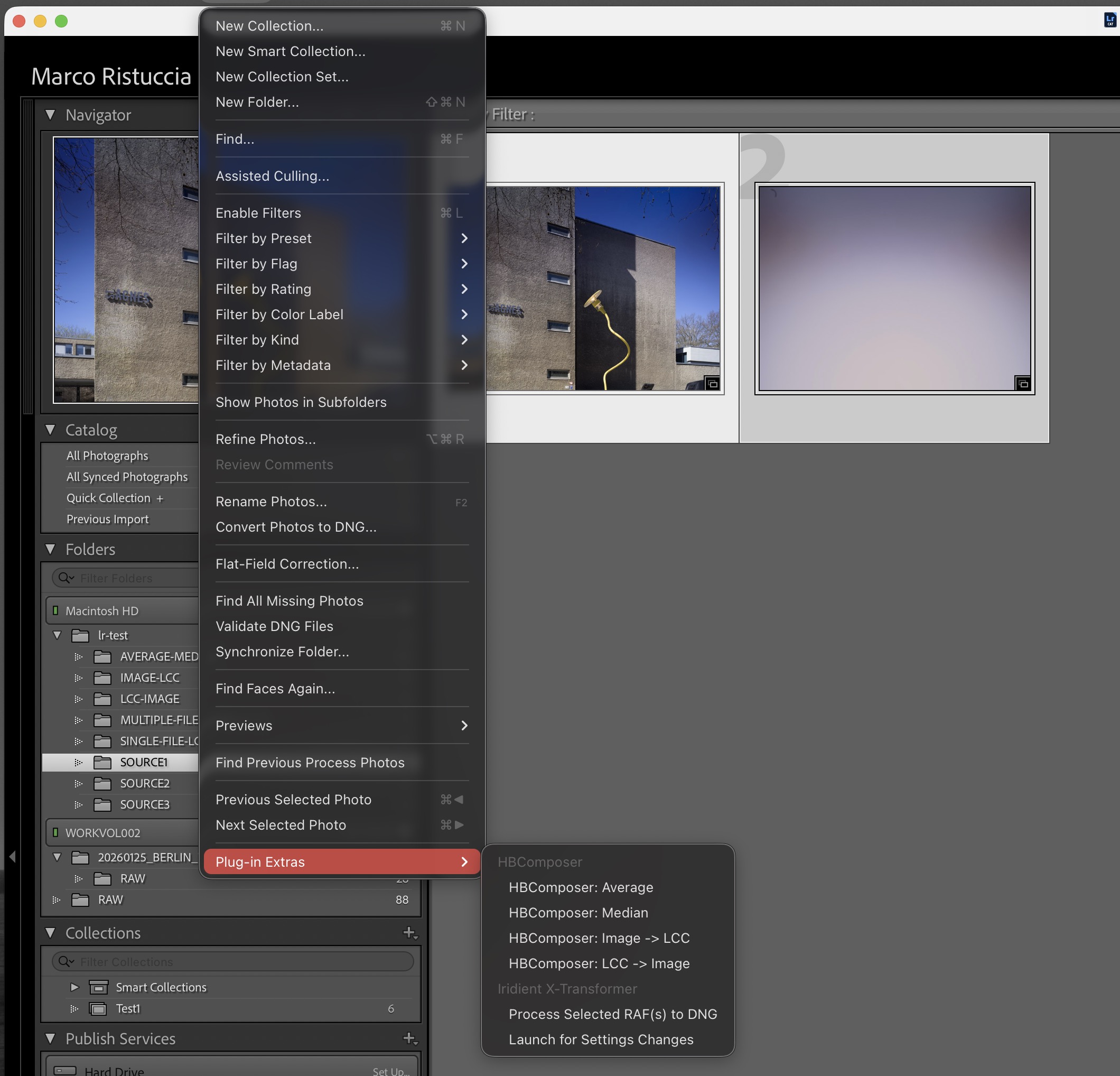
Before executing any action, the files that the action applies to must be selected from the Lr Library Grid.
Below is a brief description of the actions provided.
Average: a frame-average of the selected images will be produced. If the configuration checkbox Align frames… is enabled, an automatic frame pre-alignment is performed before composing the files. See more in Frame-Average.
Median: a frame-median of the selected images will be produced. If the configuration checkbox Align frames… is enabled, an automatic frame pre-alignment is performed before composing the files. See more in Frame-Median.
Image -> LCC: For each image, the LCC immediately following it in the Lr grid is applied. Therefore, the number of selected images must be even and the images must be organized in the grid so that each LCC frame follows its matching image. More in this in Operations and flat-field correction.
LCC -> Image: For each image, the LCC immediately preceding it in the Lr grid is applied. Therefore, the number of selected images must be even and the images must be organized in the grid so that each LCC frame precedes its matching image. More on this in Operations and flat-field correction.
Some caveats:
The plugin works on both real folders and collections. The processed images appear automatically. If they won’t, probably an old one is already there. In such case, a folder sync in Lr followed by an inspection and eventually a removal of the old file may be needed before running the action again.
When working in a collection with Average and Median actions, the produced image (FA.3FR / FM.3FR) will be physically placed in the same folder as the first image in the selected series.
When working in a collection with the Image -> LCC action, each corrected image produced (…_HBG.3FR) will be physically placed in the same folder as the corresponding original image.
When working in a collection with the Image -> LCC action, each corrected image produced (…_HBG.3FR) will be physically placed in the same folder as the corresponding LCC image.
Plugin uninstallation
The plugin is uninstalled via HBComposer:
Launch HBComposer.
Open the Help menu and select Uninstall Lightroom Plugin… (see Figure 27).
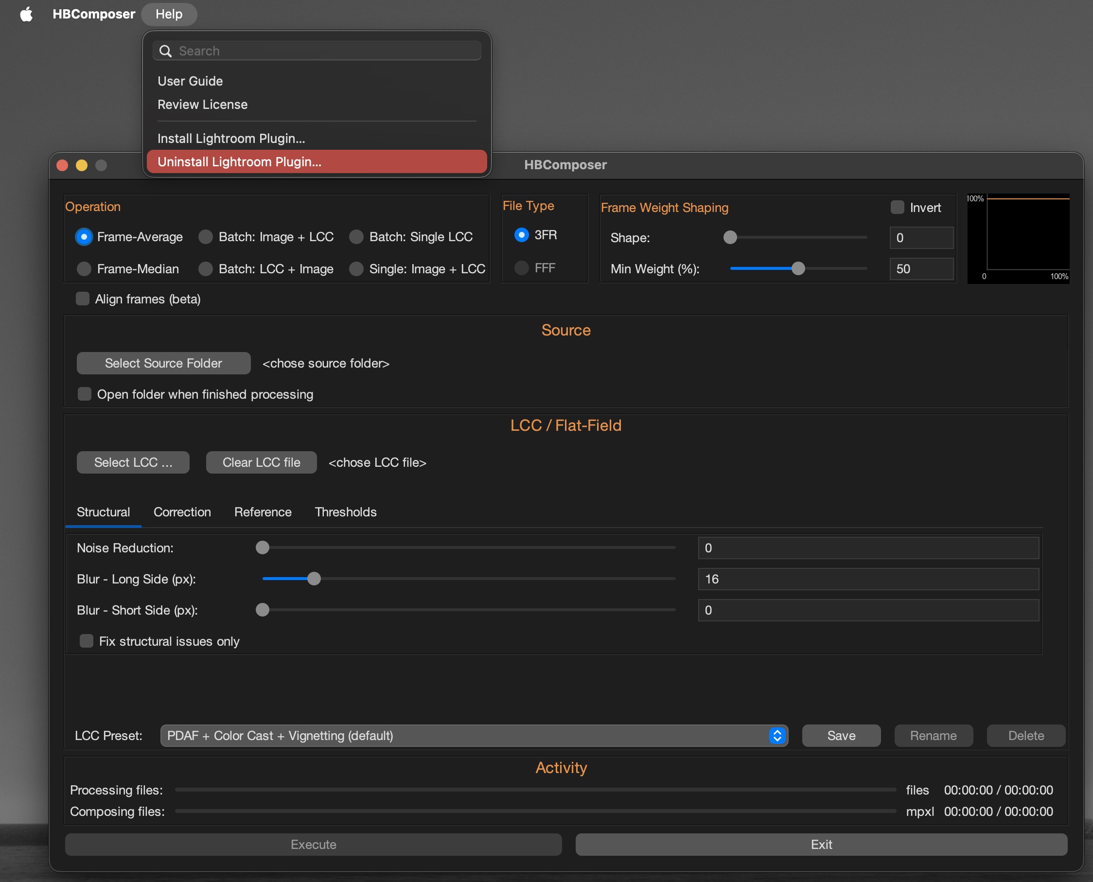
Figure 27. HBComposer – Uninstall Lightroom plugin After a confirmation request, the plugin will be automatically removed. A dialog box will confirm the removal (see Figure 28).
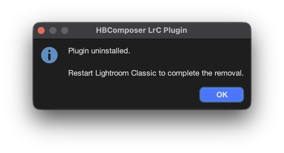
Figure 28. HBComposer – Plugin uninstallation result To complete the removal, a Lightroom restart is needed if it was already running while uninstalling the plugin.